Useful basic signals

ASP in python: 2

Dec 08, 2023

Generating some elementary signals can come in handy to test algorithms, synthesise new signals, and play around with ASP. Let’s begin with importing the required python libraries.

# import libraries/modules
import numpy as np
import matplotlib.pyplot as plt
from scipy import signal as sg

Delta signal (unit impulse)

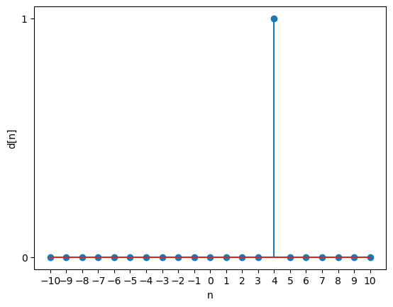
A unit delta signal has a value 1 for a specified index and 0 at all other indices.

\(\delta[n-a] = \begin{cases} 1,& \text{for } n= a\\ 0 & \text{otherwise} \end{cases}\)

To generate this signal, we need to first specify the upper limit (UL) and lower limit (LL) of the indices over which the signal is spread.

# defining parameters
a = 4
UL = 10
LL = -10
n = np.arange(LL, UL+1, 1)

# generating signal 
delta =[]
for sample in n:
        if sample == a:
            delta.append(1)
        else:
            delta.append(0)

# plotting the signal
plt.stem(n,delta)
plt.xticks(n)
plt.yticks([0, 1])
plt.xlabel('n')
plt.ylabel('d[n]')
plt.show()

Unit step

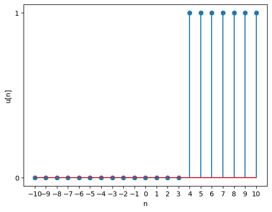
A unit step function has a value of 1 for all indices above a specified value, and 0 for all indices below that value.

\(u[n-a] = \begin{cases} 1,& \text{for } n\geq a\\ 0 & \text{otherwise} \end{cases}\)

# defining parameters
a = 4
UL = 10
LL = -10
n = np.arange(LL, UL+1, 1)

# generating signal
unit =[]
for sample in n:
    if sample<a:
        unit.append(0)
    else:
        unit.append(1)

# plotting the signal
plt.stem(n,unit)
plt.xticks(n)
plt.yticks([0, 1])
plt.xlabel('n')
plt.ylabel('u[n]')
plt.show()

Unit ramp

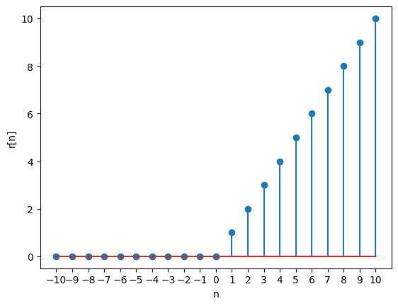
This signal starts at t = 0 and increases linearly with time with a slope of 1.

\(r[n] = \begin{cases} n,& \text{for } n\geq 0\\ 0 & \text{otherwise} \end{cases}\)

# defining parameters
UL = 10
LL = -10
n = np.arange(LL, UL+1, 1)

# generating signal
ramp =[]
for sample in n:
    if sample<0:
        ramp.append(0)
    else:
        ramp.append(sample)

# plotting the signal
plt.stem(n,ramp)
plt.xticks(n)
plt.xlabel('n')
plt.ylabel('r[n]')
plt.show()

Exponential signal

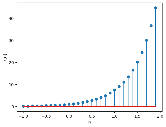
This signal is given by:

\(x[n] = e^{an}\)

# defining parameters
a = 2
UL = 1
LL = -1
n = np.arange(LL, UL+1, 0.1)

# generating signal
expo = np.exp(a * n)

# plotting the signal
plt.stem(n,expo)
plt.xlabel('n')
plt.ylabel('x[n]')
plt.show()

Exponential decay

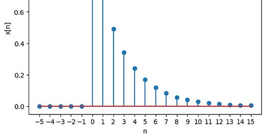
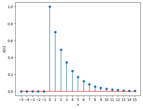
This signal starts at index 0 and decays exponentially with a factor a.

\(x[n] = |a|^n \ u[n]; a \leq 1\)

# defining parameters
a = 0.7
UL = 15
LL = -5
n = np.arange(LL, UL+1, 1)

# generating unit step signal
unit =[]
for sample in n:
    if sample<0:
        unit.append(0)
    else:
        unit.append(1)
# generating exponential decay signal
x = (a**n) * unit

# plotting the signal
plt.stem(n,x)
plt.xticks(n)
plt.xlabel('n')
plt.ylabel('x[n]')
plt.show()

Parameters for periodic signals

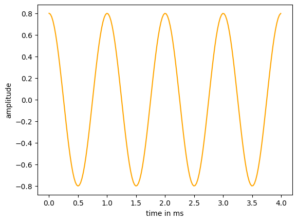
We will define the amplitude A, frequency f, initial phase phi, and sampling frequency fs. We will also generate time values over a 4-millisecond duration or 177 samples at a sampling frequency of 44100 Hz.

# defining parameters
A = 0.8
f = 1000
phi = np.pi/2
fs = 44100

n = np.arange(0,177) # 177 samples
t = n/fs

'''
alternatively,
# generating timestamps using t = nT = n/fs
t = np.arange(0,.004,1.0/fs) # duration 4 milliseconds
'''

Sine wave

We want to generate a sine wave of the form

\(x[n] = A\ sin(ωnT+\phi)=A\ sin(2πfnT+\phi)\)

where A is the amplitude, f is frequency in Hertz, T is the sampling period in seconds (inverse of sample rate fs), n is the time index, ω is the angular frequency in radian/second, and ϕ is the initial phase of the signal in radians.

# generating signal
x = A * np.sin(2*np.pi*f*t+phi)


# converting time to milliseconds for plotting
t1 = t*1000
# plotting the signal
plt.plot(t1,x, color='orange')
plt.xlabel('time in ms')
plt.ylabel('amplitude')
plt.show()

Square wave

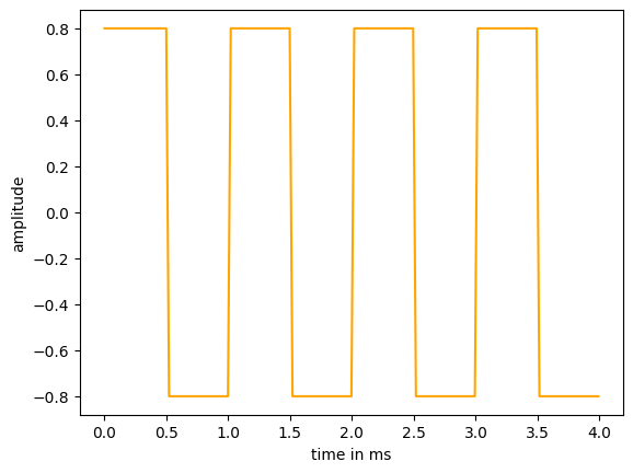
The argument duty defines the duty cycle of the wave, which is the ratio of time a load or circuit is ON (‘high’ state of the square wave) compared to the time the load or circuit is OFF (‘low’ state of the square wave). It must be in the interval [0,1].

# generating signal
# see imports (sg)
x = A*sg.square(2*np.pi*f*t, duty=0.5)

# converting time to milliseconds for plotting
t1 = t*1000
# plotting the signal
plt.plot(t1,x, color='orange')
plt.xlabel('time in ms')
plt.ylabel('amplitude')
plt.show()

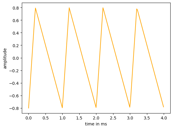
Sawtooth wave

The argument width specifies the ratio of time the wave rises. It must be in the interval [0,1].

# generating signal
# see imports (sg)
x = A*sg.sawtooth(2*np.pi*f*t, width=0.2)

# converting time to milliseconds for plotting
t1 = t*1000
# plotting the signal
plt.plot(t1,x, color='orange')
plt.xlabel('time in ms')
plt.ylabel('amplitude')
plt.show()

Thank you for reading Gannygit. This post is public so feel free to share it.

Gannygit